Chapter 4 Models in R
4.1 Packages required for this chapter
For this chapter you need to have the tidyverse, broom and MuMIn packages installed.
This chapter will explain how to generate models in R, how to obtain information and tables from models with the Broom package (Robinson and Hayes 2018) and a brief introduction to model selection with the MuMIn package (Barton 2018 )
This class of the course can also be followed at this link.
4.2 Statistical models
A statistical model tries to explain the causes of an event based on a sample of the total population. The assumption is that if the sample we obtain from the population is representative of it, we will be able to infer the causes of the population variation by measuring explanatory variables. In general, we have a response variable (the phenomenon we want to explain), and one or more explanatory variables that would deterministically generate part of the variability in the response variable.
4.2.1 Example
Let’s take the example of the CO2 database present in R (Potvin, Lechowicz, and Tardif 1990). Suppose we are interested in knowing what factors affect the uptake of \(CO_2\) in plants.
| Plant | Type | Treatment | conc | uptake |
|---|---|---|---|---|
| Qn1 | Quebec | nonchilled | 95 | 16.0 |
| Qn1 | Quebec | nonchilled | 175 | 30.4 |
| Qn1 | Quebec | nonchilled | 250 | 34.8 |
| Qn1 | Quebec | nonchilled | 350 | 37.2 |
| Qn1 | Quebec | nonchilled | 500 | 35.3 |
| Qn1 | Quebec | nonchilled | 675 | 39.2 |
| Qn1 | Quebec | nonchilled | 1000 | 39.7 |
| Qn2 | Quebec | nonchilled | 95 | 13.6 |
| Qn2 | Quebec | nonchilled | 175 | 27.3 |
| Qn2 | Quebec | nonchilled | 250 | 37.1 |
| Qn2 | Quebec | nonchilled | 350 | 41.8 |
| Qn2 | Quebec | nonchilled | 500 | 40.6 |
| Qn2 | Quebec | nonchilled | 675 | 41.4 |
| Qn2 | Quebec | nonchilled | 1000 | 44.3 |
| Qn3 | Quebec | nonchilled | 95 | 16.2 |
| Qn3 | Quebec | nonchilled | 175 | 32.4 |
| Qn3 | Quebec | nonchilled | 250 | 40.3 |
| Qn3 | Quebec | nonchilled | 350 | 42.1 |
| Qn3 | Quebec | nonchilled | 500 | 42.9 |
| Qn3 | Quebec | nonchilled | 675 | 43.9 |
In the table 4.1 we see the first 20 observations of this database. We see that within the factors we have to explain the capture of \(CO_2\) are:
- Type: Subspecies of plant (Mississippi or Quebec)
- Treatment: Plant treatment, chilled or nonchilled
- conc: Environmental concentration of \(CO_2\), in mL/L.
A possible explanation that would allow us to try to explain this phenomenon is that the plants of different subspecies will have different uptake of \(CO_2\), which we explore in the graph 4.1:
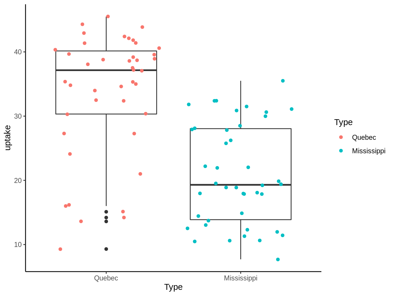
Figure 4.1: CO2 uptake by plants dependent on their subspecies
We see that there is a tendency for plants originating in Quebec to capture more \(CO_2\) than those from the Mississippi, but can we effectively say that both populations have different means? That’s where models come in.
4.2.2 Representing a model in R
In R most models are represented with the following code:
some_function(Y ~ X1 + X2 + ... + Xn, data = data.frame)In this model, we have the response variable Y, which can be explained by one or multiple explanatory variables X, that is why the symbol ~ reads explained by, where what is on its left is the response variable and to the right the explanatory variable. The data is in a data frame and finally we will use some function, which will identify some model. Some of these functions are found in the table 4.2
| Modelos | Funcion |
|---|---|
| t-test | t.test() |
| ANOVA | aov() |
| Linear model | lm() |
| Generalized linear model | glm() |
| Generalized aditive model | gam() |
| non-linear model | nls() |
| Mixed effect models | lmer() |
| Boosted regression trees | gbm() |
4.2.3 Let’s go back to the example of plants
For this example we will use a simple linear model, for this following the table 4.2 lets use the lm function:
Fit1 <- lm(uptake ~ Type, data = CO2)4.2.3.1 Using broom to get more out of your model
the broom package (Robinson and Hayes 2018) is a package adjacent to the tidyverse (so you have to load it separately from the tidyverse), which allows us to take information from models generated in tidy format. Today we will look at 3 broom functions, these are glance, tidy and augment.
4.2.3.1.1 glance
The glance function will give us general information about the model, such as the p value, the \(R^2\), log-likelihood, degrees of freedom, and/or other parameters depending on the model to be used. This information is delivered to us in a data frame format, as we see in the following code and in the table 4.3
library(broom)
glance(Fit1)| r.squared | adj.r.squared | sigma | statistic | p.value | df | logLik | AIC | BIC | deviance | df.residual | nobs |
|---|---|---|---|---|---|---|---|---|---|---|---|
| 0.346713 | 0.3387461 | 8.794012 | 43.5191 | 0 | 1 | -300.8007 | 607.6014 | 614.8939 | 6341.441 | 82 | 84 |
4.2.3.1.2 tidy
the tidy function will give us information about the model parameters, that is the intercept, the slope and/or interactions, as we see in the following code and in the table 4.4
tidy(Fit1)| term | estimate | std.error | statistic | p.value |
|---|---|---|---|---|
| (Intercept) | 33.54286 | 1.356945 | 24.719384 | 0 |
| TypeMississippi | -12.65952 | 1.919011 | -6.596901 | 0 |
4.2.3.1.3 augment
The augment function will give us, for each observation of our model, several important parameters such as the predicted value, the residuals, the cook distance, among others, this mainly serves us to study the assumptions of our model. Below we see the use of the augment function and 20 of its observations in the table 4.5
augment(Fit1)| uptake | Type | .fitted | .resid | .hat | .sigma | .cooksd | .std.resid |
|---|---|---|---|---|---|---|---|
| 28.5 | Mississippi | 20.88333 | 7.6166667 | 0.0238095 | 8.806572 | 0.0093715 | 0.8766185 |
| 15.1 | Quebec | 33.54286 | -18.4428571 | 0.0238095 | 8.601612 | 0.0549457 | -2.1226279 |
| 41.4 | Quebec | 33.54286 | 7.8571429 | 0.0238095 | 8.803900 | 0.0099726 | 0.9042954 |
| 19.4 | Mississippi | 20.88333 | -1.4833333 | 0.0238095 | 8.846557 | 0.0003554 | -0.1707200 |
| 37.2 | Quebec | 33.54286 | 3.6571429 | 0.0238095 | 8.838566 | 0.0021605 | 0.4209084 |
| 11.3 | Mississippi | 20.88333 | -9.5833333 | 0.0238095 | 8.782250 | 0.0148358 | -1.1029663 |
| 34.8 | Quebec | 33.54286 | 1.2571429 | 0.0238095 | 8.847000 | 0.0002553 | 0.1446873 |
| 27.8 | Mississippi | 20.88333 | 6.9166667 | 0.0238095 | 8.813874 | 0.0077281 | 0.7960540 |
| 7.7 | Mississippi | 20.88333 | -13.1833333 | 0.0238095 | 8.723037 | 0.0280755 | -1.5172980 |
| 38.7 | Quebec | 33.54286 | 5.1571429 | 0.0238095 | 8.829102 | 0.0042963 | 0.5935466 |
| 41.8 | Quebec | 33.54286 | 8.2571429 | 0.0238095 | 8.799269 | 0.0110138 | 0.9503322 |
| 30.4 | Quebec | 33.54286 | -3.1428571 | 0.0238095 | 8.841068 | 0.0015956 | -0.3617181 |
| 30.9 | Mississippi | 20.88333 | 10.0166667 | 0.0238095 | 8.776132 | 0.0162078 | 1.1528396 |
| 30.0 | Mississippi | 20.88333 | 9.1166667 | 0.0238095 | 8.788531 | 0.0134261 | 1.0492567 |
| 34.6 | Quebec | 33.54286 | 1.0571429 | 0.0238095 | 8.847331 | 0.0001805 | 0.1216688 |
| 19.9 | Mississippi | 20.88333 | -0.9833333 | 0.0238095 | 8.847439 | 0.0001562 | -0.1131739 |
| 42.9 | Quebec | 33.54286 | 9.3571429 | 0.0238095 | 8.785334 | 0.0141437 | 1.0769336 |
| 32.4 | Mississippi | 20.88333 | 11.5166667 | 0.0238095 | 8.752828 | 0.0214255 | 1.3254778 |
| 35.0 | Quebec | 33.54286 | 1.4571429 | 0.0238095 | 8.846612 | 0.0003430 | 0.1677057 |
| 18.1 | Mississippi | 20.88333 | -2.7833333 | 0.0238095 | 8.842591 | 0.0012514 | -0.3203398 |
4.2.3.2 Model selection using broom and the AIC
The AIC, or Akaike Information Criterion (Aho, Derryberry, and Peterson 2014), is a measure of how much information a model gives us given its complexity. This last measure from the number of parameters it has. The lower the AIC, the comparatively better a model is, and in general, a model that is two AIC units lower than another model will be considered a model that is significantly better than another.
The Akaike selection criterion formula is the one we see in the equation (4.1).
\[\begin{equation} AIC = 2 K - 2 \ln{(\hat{L})} \tag{4.1} \end{equation}\]
Where \(K\) is the number of parameters, which we can see with tidy, if we look at the table 4.4, we see that the model Fit1 has 2 parameters, that is \(K\) is equal to 2 .
The log-likelihood of the model (\(\ln{(\hat{L})}\)) is the fit it has to the data. The more positive this value is, the better the model fits the data, and the more negative it is, the less it fits the data. In our model, using glance, we can see that the model’s log-likelyhood value is -300.8 (see table 4.4).
Therefore, substituting the equation (4.1), we obtain 605.6, which is a value very close to the 608, which appear in the model’s glance (table 4.4).
4.2.3.2.1 Candidate Models
Let’s look at the figure 4.2. to think about what might be interesting models to explore.
ggplot(CO2, aes(x = conc, y = uptake)) + geom_point(aes(color = Type,
    shape = Treatment), size = 3)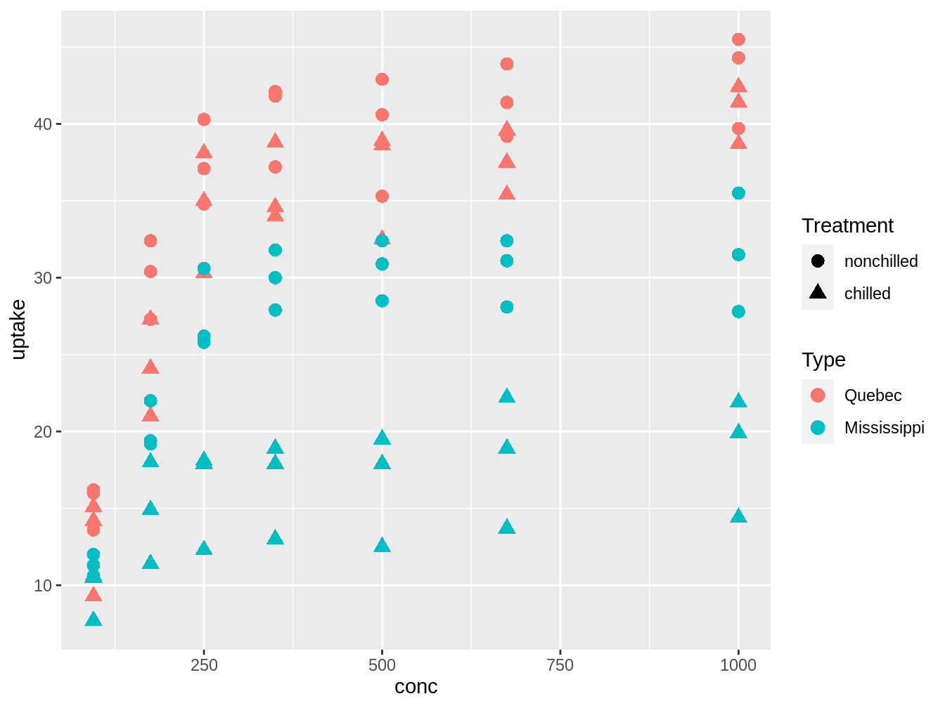
Figure 4.2: Exploratory graph to generate models from the CO2 database